A while back, Antmicro introduced an open source-driven flow for thermal simulation using finite element analysis (FEA), later enhanced with improved convection calculations. The thermal simulations we have showcased so far demonstrated optimal performance with simple, single-body models and simulations of natural convection or radiative heat transfer in vacuum. FEA is great for quick, lightweight simulations in the time domain. However, for complex, multi-part designs, detailed geometries or forced convection characterized with turbulent air flow, setting up boundary conditions for every surface becomes cumbersome. Additionally, FEA does not simulate the surroundings of the object, making the simulation of heat transfer between multiple objects inaccurate.
In order to simulate heat transfer between multiple objects and turbulent flows characteristic for active cooling, we expanded our thermal simulation flow with a new methodology based on Computational Fluid Dynamics (CFD). It simulates not only the temperature inside the solid, but also the temperature and flow of the surrounding fluid. From the physical perspective, this also applies to systems that utilize air or gas as a coolant. This approach eliminates the need to manually estimate complex surface heat dissipation coefficients and enables multi-object heat transfer simulations.
In this article, we will describe the workflow for a steady-state simulation of conjugate heat transfer in complex designs and show how we use it to predict and visualize temperature gradient and air velocity. We will illustrate this approach using a setup consisting of the Antmicro baseboard for NVIDIA Jetson AGX Thor, the NVIDIA Jetson AGX Thor SoM, a heat-sink, two fans, and our custom ruggedized enclosure as an example.
CFD-based thermal simulation flow
Antmicro developed a set of scripts for simulating steady-state conjugate heat transfer in complex designs using OpenFOAM, automating the analysis pipelines for creating static visualizations of the OpenFOAM simulation results in ParaView, and animating them in Blender.
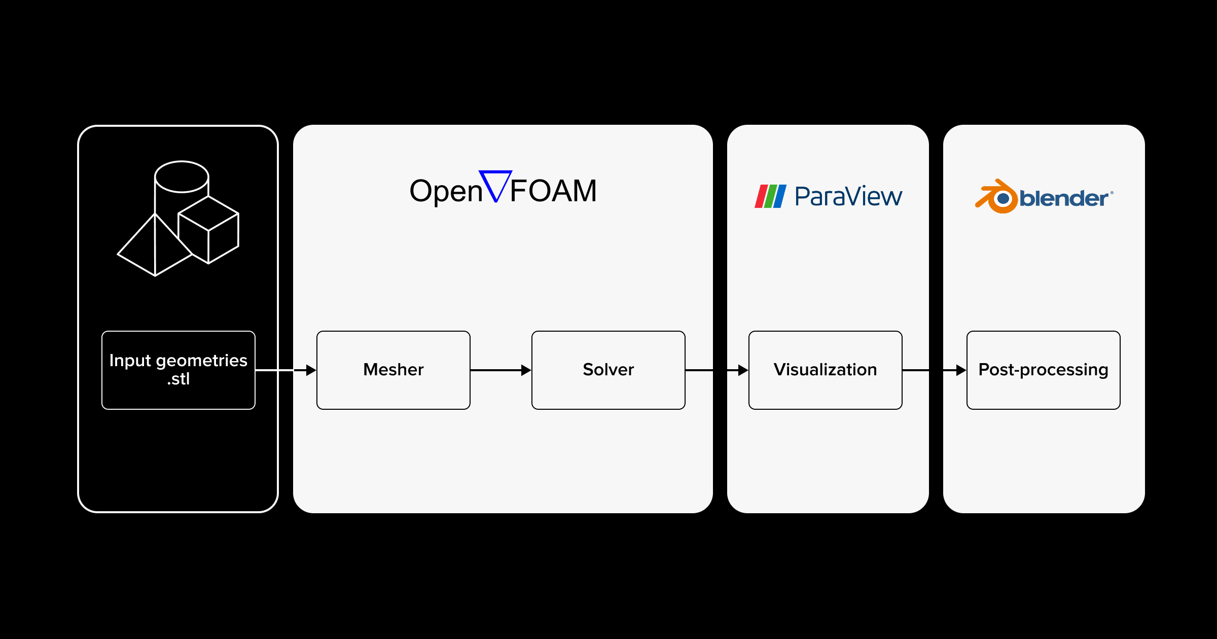
Antmicro’s CFD-based thermal simulation flow consists of the following steps:
Preparing geometries for OpenFOAM
In order to prepare a valid model consisting of multiple geometries, each of them needs to be exported as a separate .stl file. A geometry must be a closed surface without any non-manifold edges. OpenFOAM requires all dimensions to be provided in SI units.
Analysis in OpenFOAM
To perform an analysis in OpenFOAM, the following steps must be completed. First, the input geometry must be meshed, which involves creating a computational domain composed of small cells and assigning them to the corresponding regions. Next, the physics properties, such as initial conditions, heat and fluid motion sources, and material properties need to be defined. Finally, the numerical methods used to solve the equations within the computational domain must be specified in order to properly configure the solver.
For more information on how to configure your case in OpenFOAM, see the README.
After completing the above steps, you can run the simulation. During this phase the partial differential equations representing the conservation of mass, momentum and energy are solved based on the defined physical properties within the particular mesh cell volumes. The analysis results in velocity, temperature and pressure fields for every cell.
Result visualization in ParaView
Simulation results are visualized automatically with post-processing scripts that utilize ParaView. Solids are colored according to their absolute temperature fields, while fluid is visualized with streamlines that reflect the magnitude and direction of the velocity vectors. At the end, all objects are exported as glTF files. For more advanced visualization that incorporates contour plots, vector glyphs or isosurfaces, previewing simulation results in the ParaView GUI and applying the desired filter is recommended.
Post-processing in Blender
Post-processing scripts fully automate the process of animating the thermal steady state. Visualization of the temperature field is achieved by applying a color map to solid objects through Blender materials. Fluid flow is animated with Blender geometry nodes that generate discrete air cubics moving along the streamlines. To configure the camera and lights of the scene and render the frames, Antmicro’s PCBooth is used. After rendering, the animation frames are combined using ffmpeg.
For detailed instructions and complete simulation examples, visit the cfd-simulation-scripts repository.
Example use case: simulating thermal performance of NVIDIA Jetson AGX Thor
In order to illustrate the flow outlined above, we applied it to a ruggedized NVIDIA Jetson AGX Thor Baseboard setup composed of a complex, CNC-milled enclosure we designed and our open hardware baseboard for NVIDIA Jetson AGX Thor.
The detailed mechanical bill of mechanical parts used for the simulation setup was:
- NVIDIA Jetson AGX Thor SoM
- Antmicro’s baseboard for NVIDIA Jetson AGX Thor
- Anodized aluminum enclosure
- Copper heat-sink placed inside the aluminum enclosure
- 3-D printed fan shroud
- 2 x blower-type fans
Mesh adjustments
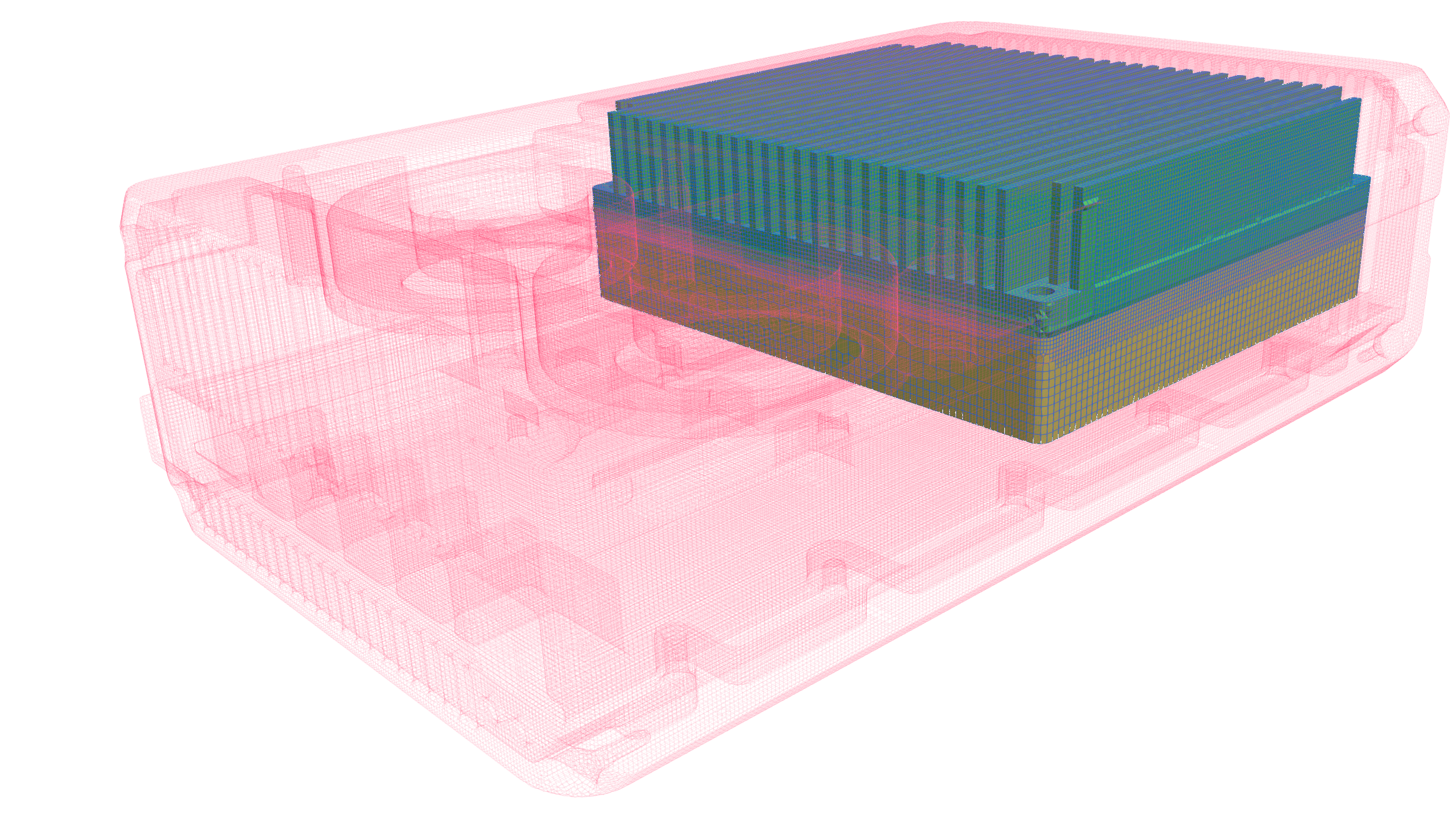
We increased the mesh resolution in regions with high air velocity, specifically the heat-sink fins, to enhance simulation accuracy. The outside of the enclosure has a lower mesh refinement level. This targeted approach provides high local mesh resolution only where it is needed. As a result, the global mesh size does not increase unnecessarily, preventing excessive computational cost.
Simulation setup
The simulated model has been defined by assigning thermophysical properties to all computational domains as follows: aluminum for the SoM and the enclosure, copper for the heat-sink, and air for the fluid domain. The thermal load of 110W generated by the SoM is represented as a uniform volumetric heat source distributed across its cells. The heat source is increased gradually from zero to target power at the beginning of the simulation to prevent numerical instability.
The airflow from each blower is modeled using momentum sources applied to the corresponding outlet cell zones. Within these zones, the air velocity is dynamically adjusted to the local static pressure gradient, calculated on the basis of the blower’s documentation. Due to the high mesh density, low under-relaxation factors were applied to enhance convergence speed while maintaining numerical stability.
Simulation results

The plot represents the simulation’s solver path, as a function of the simulation steps, up to the point of stabilized operation. The value at which it stabilizes is the steady-state simulation result. In this specific case, the value was reached after 13k iterations, and corresponds to 150.8/66 °F/°C at the SoM enclosure.
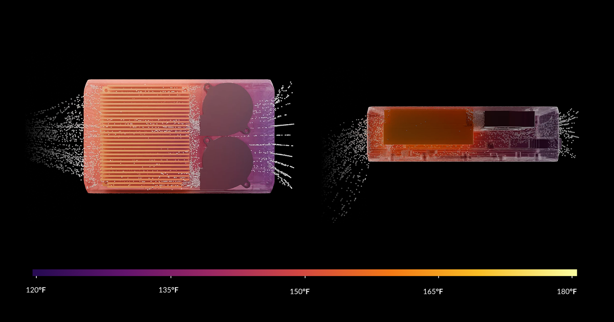
The visualization represents fluid whirlwinds, fluid motion and temperature gradient across the model. There is no temperature bottleneck between the Jetson Thor SoM and the heat-sink, as the SoM has lower conductivity (aluminum) than the heat-sink (copper). Part of the heat-sink outlet air recirculates back to the bottom of the fans via a channel beneath the heat-sink and the Thor SoM. The ability to detect such issues at an early stage helps us to eliminate errors before production and to test different variants in order to optimize the design.
Verification of the simulation results with real-life measurement
To validate the accuracy of the CFD simulations, thermal characterization tests were conducted on the physical mechanical assembly integrated with the Jetson Thor SoM. The primary objective was a comparison of theoretical heat dissipation patterns with real-world measurement of the module under high-load conditions.

During the bench test, as the SoM temperature stabilized, the SoM power draw was 110W. The temperature of the SoM was monitored with its internal sensors and externally mounted probes.
The temperature measured on the SoM’s thermal transfer plate (TTP) stabilized at 147.9/64.4 °F/°C.
The simulation applies to the TTP and does not cover the internal structure of the SoM and its workload dynamics. Based on NVIDIA’s Jetson Thor Series Modules Thermal Design Guide p.5 and the simulation results, we’ve calculated the expected SoC temperature to be 186.4/85.8 °F/°C. Measurements of the internal temperature, obtained using the tegrastats utility, showed a maximum SoC temperature of 187.9/86.6 °F/°C.
| Measurement point | Simulation | Measurement | Relative error [%] |
|---|---|---|---|
| TTP | 150.8/66 °F/°C | 147.9/64.4 °F/°C | 1.9 |
| SoC | 186.4/85.8 °F/°C | 187.9/86.6 °F/°C | 0.8 |
Conclusion
The simulation and calculation results met the physical measurements with a 2 % margin of error, confirming the reliability of the simulation workflow. This validates the accuracy of the numerical approach and demonstrates its effectiveness for predictive thermal analysis.
This open source workflow ensures transparency and reproducibility, since all models and implementation details are publicly available. Thanks to its flexibility, it can be easily adapted to different systems, and works well with both simple and more complex designs.
Develop custom hardware with advanced cooling solutions with Antmicro
Active cooling is omnipresent in devices that offer high computational power, such as data center nodes, high framerate/high resolution cameras and high-bandwidth communication interfaces. With the new CFD-based thermal simulation flow, Antmicro can help you develop and thoroughly test custom hardware with advanced cooling solutions.
If you would like to learn more about Antmicro’s thermal simulation solutions and other services around hardware development, reach out to us at contact@antmicro.com.